Trying to Solve Capybaradoku With Linear Algebra

Intro

Capybaradoku is a game that I made for someone so she didn’t have to watch ads on the game she liked. It’s basically a clone of LinkedIn’s Queens or Meowdoku. If you are unfamiliar, the game partitions the grid into connected colored regions. The rules are that you have to place an item (queen, cat, or capybara, depending on your variant) on a square grid so that there is only one item per row, column, and color. Also, corners of items cannot touch, so no diagonal adjacency.

Recently I was thinking that it would be fun to add some variety, and I thought about adding a hexagonal tiling mode rather than just the classic square. I’m not a math expert, but analyzing the puzzle turned out to be super interesting.

I have played the basic version quite a bit, and I’ve wondered what a solver would look like. The levels are verified by some code written by AI, but I found myself wondering if there was a better approach that didn’t involve fully permuting the search space.

Working on the hex grid, my mind jumped to linear algebra. We can set up a system of equations to describe the constraints and just solve the system with Gaussian elimination or something, was my thinking. If you are unfamiliar, Gaussian elimination is an algorithm for solving a set of linear equations.

Linear Algebra Attempt

Let’s take the 9-wide hexagonal grid, which is what we will mostly be analyzing in this write-up. There are 61 cells.

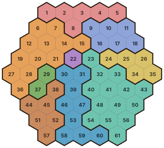
A width-9 hexagonal Capybaradoku board with 61 numbered cells grouped into nine coloured regions.

We can describe each cell as having a value of 1, meaning capybara, or 0, meaning no capybara.

In the hexagonal version of the game, a capybara can’t share any of its 3 axes with another capybara. Think of picking a hex and then going in a line from each side. Those hexes are eliminated, and each axis should still have a capybara placed.

Show one hex and its three-axis eliminations

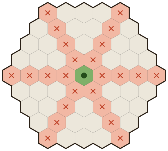
One hex highlighted in green, with every cell along its three axes marked as eliminated.

So now we can just take the cells and set up the system.

If you are unfamiliar with systems of equations, imagine setting up an equation to describe the top row of the puzzle. We know that there must be one capybara. So simply:

c_1 + c_2 + c_3 + c_4 + c_5 = 1

“The sum of all capybaras in that top row is 1.”

Then for that top-left axis you can say again:

c_1 + c_6 + c_{12} + c_{19} + c_{27} = 1

Or, “the sum of capybaras in that axis is one.”

Then for color, say green:

c_{29} + c_{37} = 1

“Green only has one capybara.”

So we can describe each constraint in the solved game. The whole board has its three axes, each with 9 constraint equations, and then there are 9 colors. So we only need

9 \times (\underbrace{3}_{\text{axes}} + \underbrace{1}_{\text{colour}}) = 36

equations.

Show one axis and its nine line-groups

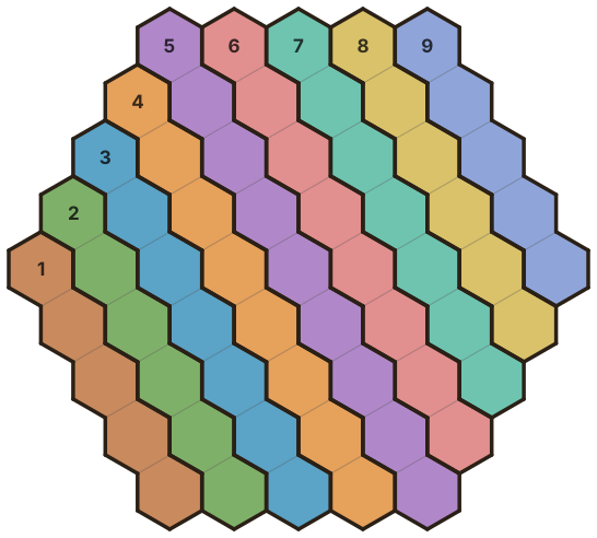
One axis direction of the board, its nine parallel lines each shown as a differently coloured group numbered 1 to 9.

Then we just solve the system of equations, which is trivial for a computer.

Which is where we run into an actually massive (literally) problem.

In this case, if you have a system of equations where there are fewer constraints than variables, there are infinitely many solutions. We have 36 constraints, our equations from earlier, and 61 variables, the number of cells. That’s not always the rule, but for Capybaradoku it is because we already know the system is consistent.

At this point I should mention that I have essentially no background in integer programming. I sort of assumed that there was a linear-algebra approach that could enforce whole-number answers. It makes clear sense to me now why that is not the case.

We are missing a key bit of information that makes this solvable.

The current mathematical representation of Capybaradoku allows for negative and fractional capybaras. Of course that would be cruel to them, to make them fractional, and I’m not sure what a negative capybara is.

We need to say that a cell can either be 0 or 1. So:

c_i \in \{0, 1\}

for every cell $i$ .

Leaving the Linear World

Fortunately, we can now solve Capybaradoku!

Unfortunately, there’s no longer an easy way to solve all the equations.

Gaussian elimination works because, over the real numbers, you can freely scale rows and add them together, and any blend of two solutions is still a solution. That freedom is exactly what gave us infinitely many answers a moment ago.

But $\{0, 1\}$ has none of that structure: add two valid boards together and you get cells equal to 2, which isn’t allowed.

The moment we demand whole-number answers, we’ve left ordinary linear algebra behind and stepped into integer programming, specifically 0–1 integer programming. General 0–1 integer programming is NP-hard, although that does not automatically mean Capybaradoku itself is NP-hard.

Well, at least we can check each possible solution against our 36 equations and verify it very quickly.

Let’s just search each possible value of each cell. That gives us the number of placements to check:

2^{61} = 2{,}305{,}843{,}009{,}213{,}693{,}952

If we check one billion possibilities per second, it will only take us over 70 years to solve the puzzle.

But that’s a rather silly approach.

We know that we can only place 9 capybaras. So we can instead search the list of ways to pick 9 cells from the total 61. This works out to:

\binom{61}{9} = 17{,}341{,}763{,}505

Now this is getting better. A computer could solve the problem this way, although it would still take a bit. And it turns out we can still do a lot, lot better.

Instead of representing the placement with a list of 61 1s and 0s, we can lean on a constraint we already have.

Each row along our reference axis needs exactly one capybara, so a whole board is completely described by which position each row’s capybara sits in.

The trick is to number those positions with a single coordinate system shared across the whole board: the same number always names the same diagonal line, so instead of every row restarting at 1, the shorter rows lower down begin above 1.

A placement then becomes a 9-tuple

(p_1, p_2, \ldots, p_9)

where $p_i$ is the coordinate of the capybara in row $i$ .

Each row still only reaches the run of coordinates that actually pass through it, so it still has exactly as many choices as it has cells: 5, then 6, 7, 8, 9, and back down.

The count of placements is unchanged.

But the shared coordinate buys us something: because a number now means the same line everywhere, the second-axis rule, “no two capybaras share that diagonal,” is just the statement that all nine $p_i$ are different.

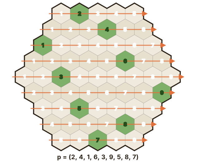
Each row of the board numbered in one shared coordinate system, with reference-axis arrows; one capybara highlighted per row and the resulting tuple written below.

Row 1 has 5 options, row 2 has 6, row 3 has 7, and so on up to 9 in the middle before shrinking back down.

Multiplying the row lengths gives the number of placements this description can express:

5 \times 6 \times 7 \times 8 \times 9 \times 8 \times 7 \times 6 \times 5 = 25{,}401{,}600

Notice that the placement numbers show a second axis, one along ones, one along twos, etc.

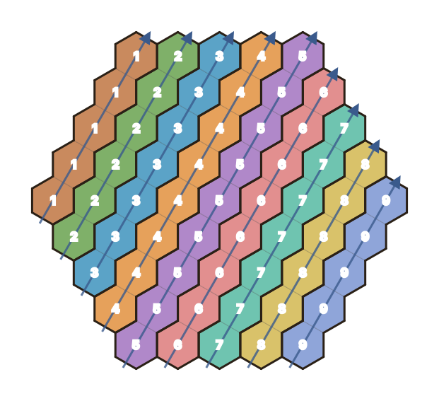
The board coloured into nine diagonal groups, one per shared coordinate value, with blue arrows running along this second axis.

There’s another constraint from this second axis: we can only pick a coordinate once.

So we can’t have something like

(1, 4, 1, \ldots)

because that would put two capybaras on the same second-axis line, both sharing the coordinate 1.

This is also why I structured the values to start at increasing numbers on the bottom four rows: it lets us easily represent the second axis and its constraint.

So that changes our search-space size again.

We can start calculating the number of options:

5 \times (6 - 1) \times (7 - 2) \times (8 - 3) \times (9 - 4) \times \cdots

For the first five rows this looks deceptively simple.

Once we get to the 6th row, though, we have a different subset of options than the first row. The number of choices left now depends on which coordinates were already used, rather than just how many.

So we can’t simply do $5^9$ .

Counting the restricted permutations that obey both axis constraints gives:

\boxed{25{,}231}

placements of 9 capybaras.

The previous image still showed a problem, though: these capybaras are sharing a third axis that we haven’t considered yet, and this is forbidden by the rules.

We can easily formalize the third-axis constraint.

So far we have been using the coordinates

(\text{row}, \text{position})

Since we are still in two dimensions, the third hexagonal axis is actually redundant: once we know the other two coordinates, the third is determined.

It is useful for creating the third-axis constraint, though, because we can calculate it from our existing coordinates and then require it to be unique just like the second axis.

With the numbering used here, the third-axis coordinate is:

s = \text{position} - \text{row} + 5

That gives us three formal rules for placing capybaras:

Unique row
Unique position
$\text{position} - \text{row} + 5$ is also unique

Applying that last constraint gets us down to just:

\boxed{244}

possible capybara placements.

If we write a program to count rotations and reflections of the board as equivalent, there are only:

\boxed{29}

fundamentally different geometric ways to place 9 capybaras on the entire 9-wide hex grid.

Conclusion

The next step is to consider the color constraints. For an actual generated Capybaradoku board with a guaranteed unique solution, those constraints ultimately reduce the remaining possibilities down to one.

There is also no separate adjacency constraint needed in the hexagonal version of the game. Any two touching hexagons already share one of the three axis lines, so satisfying all three axis constraints automatically prevents two capybaras from touching.

I did not find a general way to solve hex Capybaradoku without some form of combinatorial search. The interesting boards are designed so that the color regions reveal just enough structure for a human to reason through them instead of manually testing hundreds of placements.

That being said, defining the fixed set of geometry-valid solutions makes solving a given board enormously easier. It is also possible to sequentially generate valid placements while pruning impossible partial placements immediately, so practically this would be a huge performance boost if you were implementing a solver.

Here are the final results of the generic constraints:

Strategy	Placements for $n=9$	Scaling as board width $n$ grows
Every cell independently $0/1$	$2^{61}\approx 2.31\times10^{18}$	$2^{\Theta(n^2)}$
Choose exactly $n$ cells	$\binom{61}{9}=17{,}341{,}763{,}505$	$\binom{\Theta(n^2)}{n}$
Encode one axis	$25{,}401{,}600$	roughly $n!2^n/\sqrt n$
Enforce second axis too	$25{,}231$	at most $O(n!)$ candidates
Enforce all three axes	$\boxed{244}$	bounded above by $O(n!)$

Linear algebra did not give me the solver I initially hoped for, but it exposed the structure of the problem.

By changing how I represented the board, I was able to reduce the search space from roughly

2.3\times10^{18}

possibilities to just

244

geometry-valid placements on the 9-wide board.

That was a much more interesting result than the Gaussian-elimination solution I originally expected.

Play it

Here’s the hexagon version itself. Single-tap for a note dot, double-tap to place a capybara. Every board is generated with a guaranteed unique solution.

You can also check out the square game on capybaradoku.com if you hate ads.

Single-tap for a note dot; double-tap to place a capybara. One capybara per line along all three axes, and one per colour patch.